What Is AI Project Non-Linearity — And Why It Breaks Every Estimate You Have Ever Made

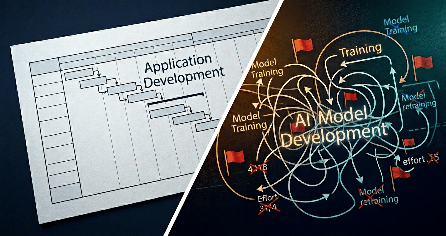
The hidden mechanics behind AI project cost overruns — and the structured approach that fixes them before the first sprint starts.

Traditional project estimation assumes effort grows linearly with complexity. AI model development does not. That single difference is responsible for more programme failures than any algorithm choice, cloud decision, or vendor selection ever will be.

Every enterprise AI programme starts with an estimate. That estimate goes into a business case. The business case gets approved. The programme starts. And at some point — usually between month two and month five — reality diverges from the estimate in ways that no risk register predicted, no contingency absorbed, and no steering committee expected.

The conventional explanation is that AI is inherently unpredictable. That is not wrong, but it is incomplete. AI projects overrun not simply because they are complex — they overrun because the estimation frameworks used to scope them were designed for a different class of problem entirely.

Software engineering estimation — whether PERT, three-point, parametric, or planning poker — was built on a foundational assumption: that effort scales roughly additively with scope. Add a feature, add some effort. Double the complexity, roughly double the timeline. This assumption holds reasonably well for deterministic systems.

Machine learning model development violates this assumption at every stage. The relationship between scope and effort is not additive. It is multiplicative. And when multiple complexity factors compound simultaneously — which they always do in real enterprise AI programmes — the result is not a 20% overrun. It is a 150% overrun.

The Concept: What Non-Linearity Actually Means in AI Delivery

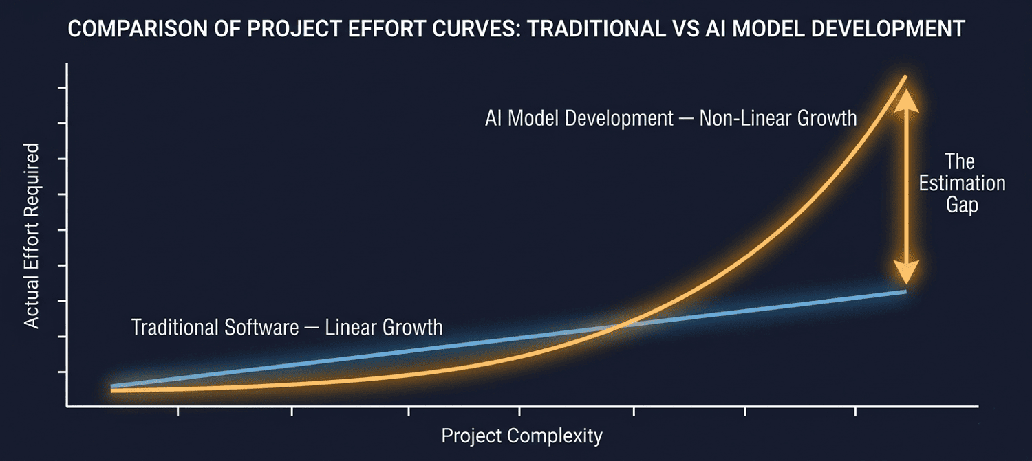
In a software project, adding a second database table to a schema takes roughly twice as long as adding the first. Adding a third takes roughly the same time as the second. The relationship between scope and effort is proportional — it is linear.

In an AI model development project, the relationship breaks down rapidly. Consider what happens when a data quality problem compounds with an architecture decision:

•       Poor data quality forces extended preprocessing — adding two to three weeks to data engineering.

•       Extended preprocessing delays the start of model training — compressing the time available for iteration.

•       Time pressure on iteration leads to shortcuts in hyperparameter tuning — producing a model that underperforms on production data.

•       Underperformance on production data triggers a root cause investigation — which reveals that the preprocessing was itself insufficient.

•       The team returns to data engineering. The cycle restarts.

No single one of these events is catastrophic. Together, they are. And crucially, none of them could have been predicted in isolation — their impact only materialises through interaction. This is the compounding structure that makes AI estimation fundamentally different from software estimation.

Non-linearity is not a risk to be managed. It is a property of the work to be measured. Treating it as a contingency item is why most AI estimates are wrong before the first sprint starts.

The practical implication is significant. A project estimated at 100 person-days under a standard software estimation framework might require 220 person-days under realistic AI delivery conditions. Not because the team is slow, not because the requirements changed, but because the multiplicative structure of AI complexity was never accounted for in the original estimate.

The Five Factors That Drive Non-Linear Effort Growth

Non-linearity in AI model development is not random. It is driven by five measurable factors. Each factor carries its own multiplier range — and when scored in combination, they produce a composite effort multiplier that reflects the true complexity of the project.

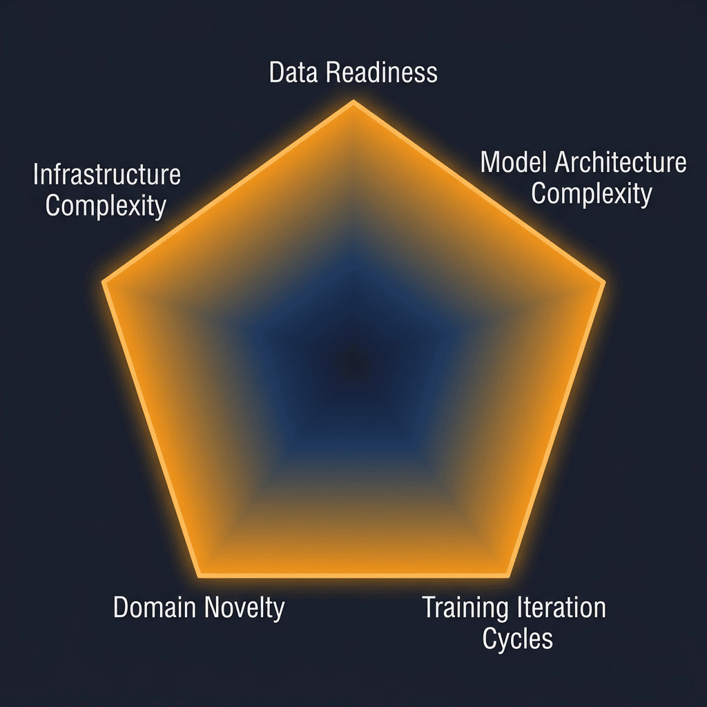
Factor 1: Data Readiness and Quality

This is, consistently, the largest driver of AI project overrun — larger than model complexity, larger than infrastructure, larger than any architectural decision the team will make. The gap between 'we have three years of historical transaction data' and 'we have production-ready, labelled, governed training data' is where months disappear.

The compounding mechanism: poor data quality does not just add preprocessing time at the start. It creates a cascade. Rushed preprocessing produces noisy features. Noisy features produce unstable models. Unstable models require more training iterations. More training iterations extend the timeline and compress the window for proper evaluation. Poor evaluation misses production failure modes. The project re-enters data engineering six weeks before go-live.

Data readiness is not a Phase 1 checkbox. It is the single most important input to your effort estimate. Score it conservatively. Always.

Factor 2: Model Architecture Complexity

There is a step-change in delivery effort between different model architecture tiers — and it is not linear. The jump from a gradient boosting classifier to a transformer-based architecture is not a 30% effort increase. It is a 50–85% effort increase on model development activities alone.

The mechanisms: transformer architectures require deeper expertise to debug when training is unstable, more compute to iterate, more careful evaluation (particularly for hallucination, distributional shift, and adversarial inputs), and significantly more documentation to satisfy governance requirements. Research-grade or fully custom architectures multiply all of these further — there is no community precedent to draw on.

Factor 3: Training Iteration Cycles

An iteration cycle is the full loop of: train the model, evaluate performance against the threshold, identify why it failed, adjust the approach, and restart. For a novel model on real-world enterprise data, three iterations is an optimistic minimum. Eight to fifteen is common. Twenty-plus occurs on complex domains with data quality issues.

The non-linearity here is not in the compute cost — it is in the human time. Each failed run requires investigation. Each investigation may surface a new data issue, a new architecture question, or a new feature engineering hypothesis. The effort per iteration does not decrease as cycles progress — it often increases, as the team works through progressively harder marginal improvement problems.

The rule of thumb: each training iteration cycle beyond three adds approximately 8% to base model development effort, compounding. At fifteen iterations, this factor alone contributes a 1.7× multiplier to Phase 3 effort.

Factor 4: Domain Novelty

Established AI domains — fraud detection, churn prediction, demand forecasting, document classification — have well-documented architectures, public benchmark datasets, accumulated practitioner knowledge, and a clear shared definition of what a good model looks like. Your team can draw on all of this.

Emerging or novel domains require the team to create that knowledge base themselves, inside your project budget. What features matter for this problem? What accuracy threshold is meaningful in this business context? What baseline are we comparing against? What does failure look like? Answering these questions through experimentation adds 15–35% to base effort before a single production model is trained.

Factor 5: Infrastructure Complexity

Cloud-managed ML platforms — AWS SageMaker in managed mode, Google Vertex AI, Azure ML with managed compute — abstract away most infrastructure decisions and substantially reduce operational overhead. This is not an endorsement of any provider; it is an acknowledgment that managed infrastructure genuinely reduces delivery risk on the infrastructure dimension.

Custom cloud architectures — multi-GPU distributed training, hybrid cloud/on-premises configurations, bespoke MLOps pipelines — add coordination overhead and debugging surface area that scales non-linearly. When something fails in a bespoke distributed training setup at 2am before a governance deadline, the resolution timeline is not 30 minutes. It is days.

How the Five Factors Compound: The Composite Multiplier

Individual factors are informative. Their compound effect is what matters for estimation. The composite non-linearity multiplier is calculated as the geometric mean of all five factor values, raised to a dampening exponent of 0.65.

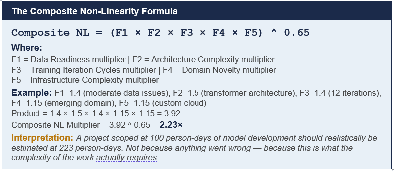
Two properties of this formula matter for how it should be used in practice.

First, the geometric mean — rather than arithmetic mean or raw multiplication — prevents any single factor from dominating the output disproportionately. A project with one extreme factor and four moderate factors should not be penalised as heavily as a project with five extreme factors. The geometric mean reflects this correctly.

Second, the 0.65 dampening exponent prevents the multiplier from reaching unrealistic extremes. Without dampening, five compounding factors at their maximum values could produce a multiplier above 10×. The dampened formula caps the practical maximum at approximately 4.5× — still significant, but reflective of the fact that not every risk materialises simultaneously at full intensity.

Non-Linearity Does Not Apply Uniformly Across Project Phases

A critical nuance that most estimation frameworks miss: non-linearity does not hit every project phase equally. The model development phase carries the full weight of non-linearity. Discovery carries almost none. Getting phase-level NL weighting right is the difference between an estimate that is accurate at the phase level and one that is directionally correct but operationally useless.

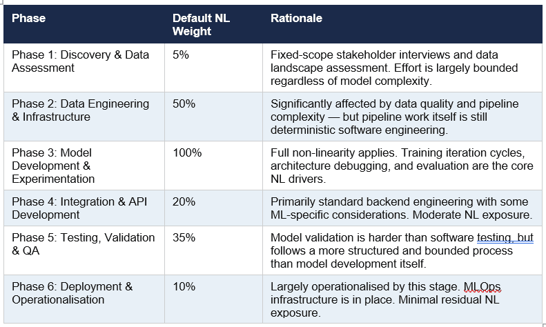
The practical consequence of phase-level weighting: applying a 2.23× composite multiplier uniformly to the entire project would overstate total effort. The same multiplier applied at full weight only to Phase 3, at 50% weight to Phase 2, and at fractional weights to the remaining phases produces a more accurate total.

Effort overestimation is as damaging as underestimation. It erodes executive confidence, creates slack that disappears into BAU, and produces business cases that do not get funded. Phase-level NL weighting is how you avoid both failure modes.

How to Interpret Your Composite Multiplier

Once the five factors are scored and the composite multiplier is calculated, the number needs to be translated into a delivery posture — not just a cost adjustment. The multiplier is not only a budget signal. It is a governance signal.

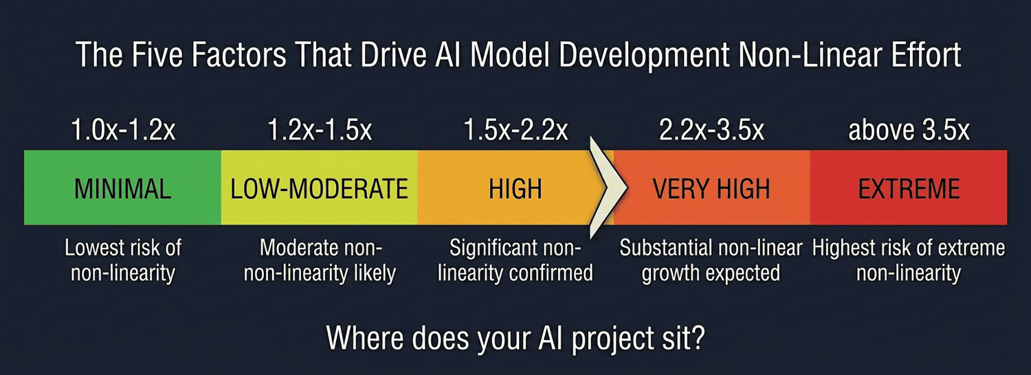
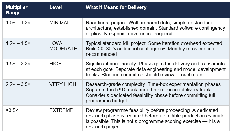
The governance implications are as important as the cost implications. A project scoring in the VERY HIGH or EXTREME band should not be approved with a single budget figure. The correct structure is staged investment — Gate 1 funds discovery and data validation, Gate 2 funds model development conditional on Gate 1 performance, Gate 3 funds production deployment conditional on Gate 2 model performance.

The mechanics of structuring a staged investment gate model for AI programmes are covered in the AI ROI Calculator guide: Staged Investment Gates for AI Programmes. The non-linearity multiplier is the primary input that determines how many gates are appropriate and where they should sit.

One Important Caveat: LLM Integration Projects Are Different

Everything described above applies specifically to AI model development — projects where your team is training, fine-tuning, or building a machine learning model from scratch or from a base model.

LLM integration projects — where your team is consuming an existing model via API (GPT-4, Claude, Gemini, Llama, and so on) and building application logic around it — follow a different effort profile. They are not subject to non-linearity multipliers in the same way. Effort scales more predictably. The primary estimation challenge is not compounding complexity in training — it is accurately forecasting token-based API costs at production volume.

Applying AI non-linearity multipliers to an LLM integration project will overstate costs by 40–80% and produce a business case that will not survive finance scrutiny. The two project types require fundamentally different estimation approaches.

The specific mechanics of LLM token cost estimation — including RAG-driven input token inflation, conversation history accumulation, and model tier selection — are covered in Blog 2 of this series: How to Estimate an AI Project Cost. A related question — why a pilot's own observed cost almost never predicts what that same system will cost at production volume — is covered separately in Why AI Pilot Costs Mislead: Estimating the Step From Pilot to Production.

AI Project Estimation Model — Viksya

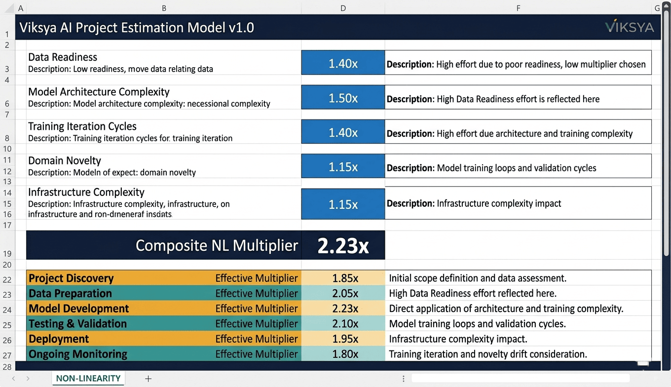
The AI Project Estimation Model from Viksya is a structured Excel-based framework that quantifies all five non-linearity factors, computes the composite multiplier automatically, and applies phase-level NL weights across a full 36-activity Work Breakdown Structure. It covers both project types — Model Development and LLM Integration — with separate cost methodologies. The output is a complete cost plan with P50, P80, and P90 confidence ranges, an AI-specific risk register, and an executive dashboard built for steering committee presentation.

→ Download the AI Project Estimation Model

Frequently Asked Questions

What is AI project non-linearity?

AI project non-linearity refers to the multiplicative — rather than additive — relationship between project complexity and delivery effort in AI model development. Unlike traditional software projects where effort scales roughly proportionally with scope, AI model development involves compounding factors — particularly data quality, training iteration cycles, and model architecture — that cause effort to grow disproportionately as complexity increases. A project twice as complex does not take twice as long; it typically takes three to five times as long.

Why do AI projects overrun their estimates so consistently?

The primary cause is the application of linear estimation frameworks to non-linear work. Traditional estimation methods — PERT, parametric models, story points — were designed for software engineering, which is broadly additive. AI model development involves five compounding complexity factors (data readiness, architecture complexity, training iterations, domain novelty, and infrastructure) that interact multiplicatively. Most AI project estimates do not account for this compounding structure, which is why overruns of 40–150% are common even on well-managed programmes.

How is the AI non-linearity multiplier calculated?

The composite non-linearity multiplier is calculated as the geometric mean of five individual factor multipliers, raised to a dampening exponent of 0.65. The formula is: Composite NL = (F1 × F2 × F3 × F4 × F5) ^ 0.65. The geometric mean prevents any single extreme factor from dominating disproportionately. The 0.65 dampening exponent prevents the multiplier from reaching unrealistic extremes in worst-case scenarios, capping the practical maximum at approximately 4.5×.

Does non-linearity apply to every phase of an AI project equally?

No. Phase 3 — Model Development and Experimentation — bears the full 100% weight of non-linearity, as it contains the core training iteration cycles and architecture decisions that drive compounding effort. Phase 1 (Discovery) bears only 5% — its effort is largely bounded by fixed-scope interviews and assessment work. Phases 2, 4, 5, and 6 carry intermediate weights of 50%, 20%, 35%, and 10% respectively. Applying the composite multiplier uniformly across all phases would overstate total project cost.

Does non-linearity apply to LLM integration projects?

No. Non-linearity multipliers apply specifically to AI model development and fine-tuning projects. LLM integration projects — where the team is building application logic around an existing model via API — have a more predictable, largely linear effort profile. The primary estimation challenge for LLM integration is accurately forecasting token-based API costs at production volume, which requires a different analytical approach.

What is a realistic non-linearity multiplier for a typical enterprise AI project?

A typical enterprise ML project with moderate data quality, a standard architecture, 8–12 training iterations, an established domain, and managed cloud infrastructure will typically produce a composite multiplier in the range of 1.4× to 1.8×. Projects with significant data quality issues, novel architectures, and emerging domains routinely produce multipliers of 2.0× to 2.8×. Research-grade or custom architecture projects can reach 3.0× to 4.5×.

How does AI project non-linearity connect to AI programme readiness?

Non-linearity multipliers are directly influenced by an organisation's AI readiness baseline — particularly data readiness, infrastructure maturity, and talent availability. Organisations that enter model development with unresolved data governance issues, unvalidated infrastructure, or insufficient ML engineering capability will consistently score higher on all five non-linearity factors. Running a structured AI readiness assessment before estimating a programme is the single most effective way to reduce non-linearity exposure upfront. Viksya's AI Transformation Readiness Scoring Model is designed for exactly this purpose: AI Transformation Readiness Scoring Model.

Related Reading from Viksya

→ How to Estimate an AI Project Cost: Model Development vs LLM Integration (Blog 2 of this series)

→ P50, P80, P90: How to Present AI Project Estimates That Get Approved (Blog 3 of this series)

→ AI Business Case Cost Modelling: The CFO-Ready Framework (AI ROI Calculator series)

→ The Six Dimensions of AI Transformation Readiness (AI Readiness Scoring Model series)